MTData: Profile Example
Now that we’ve created an MTCollection object we can use it to do the more interesting things, like analyze strike, plot phase tensors, create inputs for modeling programs.
1. Open Collection
In the previous notebook we created an MTCollection object called test_mt_collection.h5. Lets open it and get the profile.
[1]:
from pathlib import Path

from mtpy import MTCollection
[2]:
mtc = MTCollection()
mtc.open_collection(Path().cwd().joinpath("test_mt_collection.h5"))
[3]:
mtc.working_dataframe = mtc.master_dataframe.loc[
    mtc.master_dataframe.survey == "profile"
].query('station.str.startswith("15")')
[4]:
print(mtc.mt_data)
MTData Summary
  stations: 6
  surveys: 1
  lazy stations: 0
  index enabled: False
  metadata storage: cache
  dataset copy mode: shallow
  impedance units: mt
  coordinate reference frame: NED
  survey names:
    - profile
  station paths:
    - surveys/profile/stations/15125A
    - surveys/profile/stations/15126A
    - surveys/profile/stations/15127A
    - surveys/profile/stations/15128A
    - surveys/profile/stations/15129A
    - surveys/profile/stations/15130A
[5]:
mtc.working_dataframe
[5]:
| station | survey | latitude | longitude | elevation | tf_id | units | has_impedance | has_tipper | has_covariance | period_min | period_max | hdf5_reference | station_hdf5_reference | |
|---|---|---|---|---|---|---|---|---|---|---|---|---|---|---|
| 59 | 15125A | profile | -22.370806 | 149.188639 | 200.0 | 15125A | milliVolt per kilometer per nanoTesla | True | True | False | 0.000096 | 2.857143 | <HDF5 object reference> | <HDF5 object reference> |
| 60 | 15126A | profile | -22.370639 | 149.193500 | 200.0 | 15126A | milliVolt per kilometer per nanoTesla | True | True | False | 0.000096 | 2.857143 | <HDF5 object reference> | <HDF5 object reference> |
| 61 | 15127A | profile | -22.371028 | 149.198417 | 201.0 | 15127A | milliVolt per kilometer per nanoTesla | True | True | False | 0.000096 | 2.857143 | <HDF5 object reference> | <HDF5 object reference> |
| 62 | 15128A | profile | -22.370861 | 149.203306 | 200.0 | 15128A | milliVolt per kilometer per nanoTesla | True | True | False | 0.000096 | 2.857143 | <HDF5 object reference> | <HDF5 object reference> |
| 63 | 15129A | profile | -22.371083 | 149.208083 | 202.0 | 15129A | milliVolt per kilometer per nanoTesla | True | True | False | 0.000096 | 2.857143 | <HDF5 object reference> | <HDF5 object reference> |
| 64 | 15130A | profile | -22.371222 | 149.212972 | 201.0 | 15130A | milliVolt per kilometer per nanoTesla | True | True | False | 0.000096 | 2.857143 | <HDF5 object reference> | <HDF5 object reference> |
2. MTData object
MTData is an attribute of MTCollection and provides an object to work with the data. When you set working_dataframe the MTCollection.mt_data object gets updated to include only those stations withing the working_dataframe. If you want to close the collection then you can return the MTData object as follows:
[6]:
mtd = mtc.to_mt_data()
[7]:
print(mtd)
MTData Summary
  stations: 6
  surveys: 1
  lazy stations: 0
  index enabled: False
  metadata storage: cache
  dataset copy mode: shallow
  impedance units: mt
  coordinate reference frame: NED
  survey names:
    - profile
  station paths:
    - surveys/profile/stations/15125A
    - surveys/profile/stations/15126A
    - surveys/profile/stations/15127A
    - surveys/profile/stations/15128A
    - surveys/profile/stations/15129A
    - surveys/profile/stations/15130A
2a. Close MTCollection
You can now close the MTCollection to make sure if something crashes the file won’t get corrupt for unknown reasons.
[8]:
mtc.close_collection()
26:05:08T13:11:42 | INFO | line:1035 |mth5.mth5 | close_mth5 | Flushing and closing c:\Users\peaco\OneDrive\Documents\GitHub\mtpy-v2\docs\source\notebooks\test_mt_collection.h5
2b. Station Locations
A convenient attribute of MTData is the station_locations object. This is a mtpy.core.MTStations object and represented as a pandas.DataFram. You will notice here that east and north are not populated, that is because the MTData object is currently agnostic to a UTM coordinate system.
[9]:
mtd.station_locations
[9]:
| survey | station | latitude | longitude | elevation | datum_epsg | east | north | utm_epsg | model_east | model_north | model_elevation | profile_offset | |
|---|---|---|---|---|---|---|---|---|---|---|---|---|---|
| 0 | profile | 15125A | -22.370806 | 149.188639 | 200.0 | 4326 | 0 | 0 | None | 0.0 | 0.0 | 0.0 | 0 |
| 1 | profile | 15126A | -22.370639 | 149.193500 | 200.0 | 4326 | 0 | 0 | None | 0.0 | 0.0 | 0.0 | 0 |
| 2 | profile | 15127A | -22.371028 | 149.198417 | 201.0 | 4326 | 0 | 0 | None | 0.0 | 0.0 | 0.0 | 0 |
| 3 | profile | 15128A | -22.370861 | 149.203306 | 200.0 | 4326 | 0 | 0 | None | 0.0 | 0.0 | 0.0 | 0 |
| 4 | profile | 15129A | -22.371083 | 149.208083 | 202.0 | 4326 | 0 | 0 | None | 0.0 | 0.0 | 0.0 | 0 |
| 5 | profile | 15130A | -22.371222 | 149.212972 | 201.0 | 4326 | 0 | 0 | None | 0.0 | 0.0 | 0.0 | 0 |
2c. Setting UTM CRS
Its important to set the MTData.utm_crs attribute to make sure that stations can be projected into meters for plotting and creating model files. You can do this a couple of ways either through the utm_crs method or if you know the EPSG number you can input that. They should both do the same if you input the number.
If you have created a custom CRS, be sure to set mtd.utm_crs with the custom CRS.
[10]:
mtd.utm_crs = 32755
[11]:
mtd.utm_crs
[11]:
32755
[12]:
mtd.station_locations
[12]:
| survey | station | latitude | longitude | elevation | datum_epsg | east | north | utm_epsg | model_east | model_north | model_elevation | profile_offset | |
|---|---|---|---|---|---|---|---|---|---|---|---|---|---|
| 0 | profile | 15125A | -22.370806 | 149.188639 | 200.0 | 4326 | 725360.330833 | 7.524490e+06 | 32755 | 0.0 | 0.0 | 0.0 | 0 |
| 1 | profile | 15126A | -22.370639 | 149.193500 | 200.0 | 4326 | 725861.314778 | 7.524502e+06 | 32755 | 0.0 | 0.0 | 0.0 | 0 |
| 2 | profile | 15127A | -22.371028 | 149.198417 | 201.0 | 4326 | 726367.124612 | 7.524451e+06 | 32755 | 0.0 | 0.0 | 0.0 | 0 |
| 3 | profile | 15128A | -22.370861 | 149.203306 | 200.0 | 4326 | 726870.972550 | 7.524462e+06 | 32755 | 0.0 | 0.0 | 0.0 | 0 |
| 4 | profile | 15129A | -22.371083 | 149.208083 | 202.0 | 4326 | 727362.745811 | 7.524430e+06 | 32755 | 0.0 | 0.0 | 0.0 | 0 |
| 5 | profile | 15130A | -22.371222 | 149.212972 | 201.0 | 4326 | 727866.099363 | 7.524408e+06 | 32755 | 0.0 | 0.0 | 0.0 | 0 |
Now you can see that the locations have been projected into the given coordinate system.
Note: The model_east and model_north do not get populated, those are for relative coordinates for modeling.
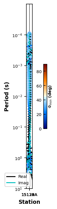
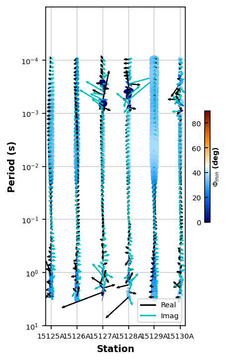
3. Plot Phase Tensor Pseudosection
Here we are adjusting the stretch in the x-direction and plotting the tipper vectors (‘r’ = real, ‘i’ = imaginary, ‘y’ = yes to plot)
[13]:
ptps_plot = mtd.plot_phase_tensor_pseudosection(x_stretch=10, plot_tipper="yri")
print(ptps_plot.x_stretch)
10
[42]:
ptps_plot.mt_data.station_locations
[42]:
| survey | station | latitude | longitude | elevation | datum_epsg | east | north | utm_epsg | model_east | model_north | model_elevation | profile_offset | |
|---|---|---|---|---|---|---|---|---|---|---|---|---|---|
| 0 | profile | 15125A | -22.370806 | 149.188639 | 200.0 | 4326 | 725360.330833 | 7.524490e+06 | 32755 | 0.0 | 0.0 | 0.0 | 0.000000 |
| 1 | profile | 15126A | -22.370639 | 149.193500 | 200.0 | 4326 | 725861.314778 | 7.524502e+06 | 32755 | 0.0 | 0.0 | 0.0 | 0.004857 |
| 2 | profile | 15127A | -22.371028 | 149.198417 | 201.0 | 4326 | 726367.124612 | 7.524451e+06 | 32755 | 0.0 | 0.0 | 0.0 | 0.009780 |
| 3 | profile | 15128A | -22.370861 | 149.203306 | 200.0 | 4326 | 726870.972550 | 7.524462e+06 | 32755 | 0.0 | 0.0 | 0.0 | 0.014665 |
| 4 | profile | 15129A | -22.371083 | 149.208083 | 202.0 | 4326 | 727362.745811 | 7.524430e+06 | 32755 | 0.0 | 0.0 | 0.0 | 0.019446 |
| 5 | profile | 15130A | -22.371222 | 149.212972 | 201.0 | 4326 | 727866.099363 | 7.524408e+06 | 32755 | 0.0 | 0.0 | 0.0 | 0.024337 |
[45]:
ptps_plot.x_stretch = 1000000
ptps_plot.redraw_plot()
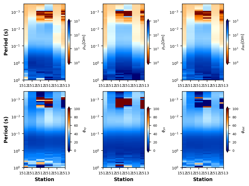
4. Plot Resistivity and Phase Pseudosections
Here we are plotting the xy, yx, and det components of the impedance tensor.
[15]:
rpps_plot = mtd.plot_resistivity_phase_pseudosections(y_stretch=700, plot_det=True)
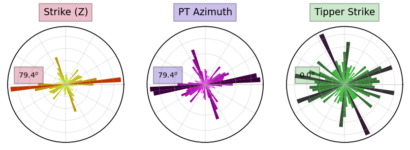
5. Plot Strike
Plotting strike angles are vary important when working with profile data. We can plot strike in a couple of ways as a compilation of all strike angles, or per decade. If you really want you could do it by region you query for the stations in each region.
5a. All Periods
Here we will plot all periods of estimated strike. Notice that the plot includes the strike as estimated from the invariants (left) of Weaver et al. (2002), the phase tensor (middel) of Caldwell et al. (2004), and the induction vector strike.
Important: The induction strike points towards good conductors so should therefore be perpendicular to the impedance strike. We left it this way as a sanity check on strike angles.
[16]:
strike_plot_all = mtd.plot_strike()
26:05:08T13:11:55 | INFO | line:860 |mtpy.imaging.plot_strike | _plot_all_periods | Note: North is assumed to be 0 and the strike angle is measured clockwise positive.
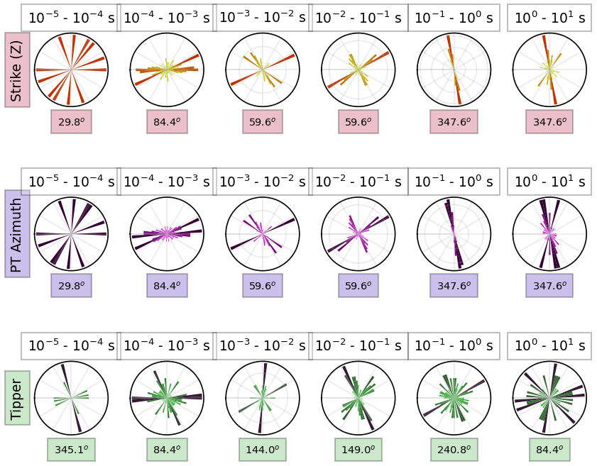
5b. Per Decade
It can be informative to plot the strike angles per decade in period. This can provide information on if strike angle changes with depth. Because this is AMT data there isn’t really a coherent strike angle until about 0.1 seconds. Notice the induction vector (tipper) strike is perpendicular to the impedance strike below 0.1 seconds.
[17]:
strike_plot_per_decade = mtd.plot_strike(plot_type=1, print_stats=True)
Strike statistics for invariant period range 1e-05 to 0.0001 (s) median=290.5 mode=0.0 mean=218.3
Strike statistics for pt period range 1e-05 to 0.0001 (s) median=290.8 mode=0.0 mean=217.8
Strike statistics for tipper period range 1e-05 to 0.0001 (s) median=35.3 mode=340.1 mean=32.6
Strike statistics for invariant period range 0.0001 to 0.001 (s) median=286.1 mode=337.7 mean=198.0
Strike statistics for pt period range 0.0001 to 0.001 (s) median=285.1 mode=337.7 mean=198.5
Strike statistics for tipper period range 0.0001 to 0.001 (s) median=1.3 mode=0.0 mean=350.6
Strike statistics for invariant period range 0.001 to 0.01 (s) median=76.4 mode=337.7 mean=156.6
Strike statistics for pt period range 0.001 to 0.01 (s) median=76.4 mode=337.7 mean=156.8
Strike statistics for tipper period range 0.001 to 0.01 (s) median=334.4 mode=59.6 mean=354.5
Strike statistics for invariant period range 0.01 to 0.1 (s) median=291.6 mode=332.7 mean=195.9
Strike statistics for pt period range 0.01 to 0.1 (s) median=291.7 mode=332.7 mean=195.8
Strike statistics for tipper period range 0.01 to 0.1 (s) median=307.4 mode=64.6 mean=338.6
Strike statistics for invariant period range 0.1 to 1 (s) median=81.5 mode=79.4 mean=93.9
Strike statistics for pt period range 0.1 to 1 (s) median=81.2 mode=84.4 mean=93.7
Strike statistics for tipper period range 0.1 to 1 (s) median=67.1 mode=153.9 mean=37.0
Strike statistics for invariant period range 1 to 10 (s) median=83.5 mode=84.4 mean=146.4
Strike statistics for pt period range 1 to 10 (s) median=79.5 mode=79.4 mean=131.6
Strike statistics for tipper period range 1 to 10 (s) median=357.9 mode=350.1 mean=5.0
26:05:08T13:11:58 | INFO | line:765 |mtpy.imaging.plot_strike | _plot_per_period | Note: North is assumed to be 0 and the strike angle is measuredclockwise positive.

6. Rotate
Rotation is common for modeling especially 2D because we want the TE mode to be parallel to the profile line and TM to be perpendicular. The strike plots above are good at indicating the dominant strike direction. From above the dominant strike direction is around N85E. There for if we want to rotate the data to a profile parallel with geoelectric strike we rotate by N85W or -85 degrees.
[18]:
mtd.rotate(-85)
6a. Plot Strike
Now if we plot the strike we see that the dominant strike is near 0. Of course you can tweek the rotation angle to get to 0, but this is close enough for demonstration purposes.
[19]:
rotated_strike = mtd.plot_strike(plot_type=1)
26:05:08T13:12:04 | INFO | line:765 |mtpy.imaging.plot_strike | _plot_per_period | Note: North is assumed to be 0 and the strike angle is measuredclockwise positive.
7. Interpolate
If you have different transfer functions processed slightly differently then you’ll likely have a mismatch in period and for modeling or plotting purposes its nice to have a single period index for all transfer functions.
You can identify the min and max from the data, if that’s what you want and then create period from there. From above it looks like the period range is from  to 0.5 seconds. Here we will interpolate onto 23 periods in that range.
[20]:
import numpy as np
[21]:
new_periods = np.logspace(-4, np.log10(0.5), 23)
[22]:
interpolated_mtd = mtd.interpolate(new_periods, inplace=False)
[23]:
interpolated_mtd
[23]:
MTData(stations=6, surveys=1, lazy_stations=0, metadata_storage='cache', dataset_copy_mode='shallow', index_enabled=False)
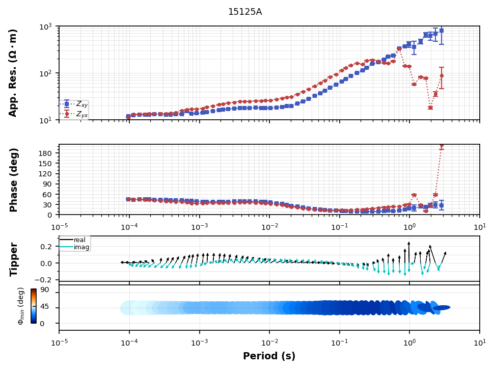
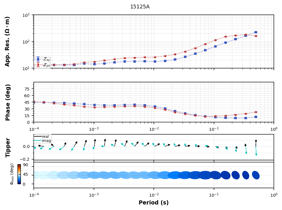
7a. Compare plots
Now we can compare to see how the interpolated transfer function compares to the original. Can plot them individually.
[24]:
original = mtd.plot_mt_response("profile.15125A")
[25]:
interpolated = interpolated_mtd.plot_mt_response("profile.15125A")
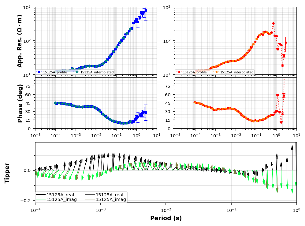
7b. Compare in same plot
To plot these in the same plot we need to do some manipulating. First change the survey name in the interpolated data. Then create a new MTData object that is just two transfer functions with the same name but from the origina and interpolated data sets.
[26]:
from mtpy.core.mt_data import MTData
from mtpy.imaging import PlotMultipleResponses
[27]:
new_interpolated_mtd = MTData()
for mt_path in interpolated_mtd.short_station_paths:
    mt_object = interpolated_mtd.get_station(mt_path, as_mt=True)
    mt_object.survey_metadata.id = "interpolated"
    new_interpolated_mtd.add_station(mt_object)
[28]:
new_interpolated_mtd.station_locations
[28]:
| survey | station | latitude | longitude | elevation | datum_epsg | east | north | utm_epsg | model_east | model_north | model_elevation | profile_offset | |
|---|---|---|---|---|---|---|---|---|---|---|---|---|---|
| 0 | interpolated | 15125A | -22.370806 | 149.188639 | 200.0 | 4326 | 725360.330833 | 7.524490e+06 | 32755 | 0.0 | 0.0 | 0.0 | 0.000000 |
| 1 | interpolated | 15126A | -22.370639 | 149.193500 | 200.0 | 4326 | 725861.314778 | 7.524502e+06 | 32755 | 0.0 | 0.0 | 0.0 | 0.004857 |
| 2 | interpolated | 15127A | -22.371028 | 149.198417 | 201.0 | 4326 | 726367.124612 | 7.524451e+06 | 32755 | 0.0 | 0.0 | 0.0 | 0.009780 |
| 3 | interpolated | 15128A | -22.370861 | 149.203306 | 200.0 | 4326 | 726870.972550 | 7.524462e+06 | 32755 | 0.0 | 0.0 | 0.0 | 0.014665 |
| 4 | interpolated | 15129A | -22.371083 | 149.208083 | 202.0 | 4326 | 727362.745811 | 7.524430e+06 | 32755 | 0.0 | 0.0 | 0.0 | 0.019446 |
| 5 | interpolated | 15130A | -22.371222 | 149.212972 | 201.0 | 4326 | 727866.099363 | 7.524408e+06 | 32755 | 0.0 | 0.0 | 0.0 | 0.024337 |
[29]:
mtd.short_station_paths
[29]:
['profile/15125A',
 'profile/15126A',
 'profile/15127A',
 'profile/15128A',
 'profile/15129A',
 'profile/15130A']
[30]:
compare_mtd = MTData()
compare_mtd.add_station(mtd.get_station("profile/15125A", as_mt=True))
compare_mtd.add_station(new_interpolated_mtd.get_station("interpolated/15125A", as_mt=True))
[30]:
'surveys/interpolated/stations/15125A'
[31]:
compare_same_plot = PlotMultipleResponses(
    compare_mtd, plot_style="compare", plot_tipper="yri", fig_num=4
)
<Figure size 640x480 with 0 Axes>
8. Occam 2D
Occam2D deGroot-Heldlin and Constable (1990) is a classic 2D inversion program. To use it you will have to compile it on your machine. For details see https://marineemlab.ucsd.edu/Projects/Occam/index.html.
Here we can create input files for Occam2D. Our data is already in an E-W profile and geoelectric strike suggests that’s a relatively good start. The dominant strike appears to be around N30W.
To get an accurate model of the data we want the profile line and the dominant geoelectric strike of the data to be perpendicular. To achieve that you can either project the stations onto a profile perpendicular to the geoelectric strike, or rotate the station data to be perpendicular to a map profile. Here, we will project the stations onto a profile perpendicular to geoelectric strike.
8a. Project stations to Geoelectric Strike
When using geoelectric strike to project stations, this is saying that the stations should project onto a profile line that is perpendicular to geoelectric strike such that when you model the data the TE mode (electric along strike) is perpendicular to the profile and the TM mode (electric perpendicular to strike) is parallel to the profile. You can read much more complete explanations looking up MT papers from the 90’s. Wannamaker et al. (1984) is a good start.
[32]:
dir(interpolated_mtd)
[32]:
['COORDINATE_REFERENCE_FRAME',
 'DATASET_COPY_MODES',
 'IMPEDANCE_UNITS',
 'METADATA_STORAGE_MODES',
 'ROOT_NAME',
 'STATIONS_NODE',
 'SURVEYS_NODE',
 '__add__',
 '__class__',
 '__deepcopy__',
 '__delattr__',
 '__dict__',
 '__dir__',
 '__doc__',
 '__eq__',
 '__firstlineno__',
 '__format__',
 '__ge__',
 '__getattribute__',
 '__getstate__',
 '__gt__',
 '__hash__',
 '__init__',
 '__init_subclass__',
 '__le__',
 '__lt__',
 '__module__',
 '__ne__',
 '__new__',
 '__reduce__',
 '__reduce_ex__',
 '__repr__',
 '__setattr__',
 '__sizeof__',
 '__static_attributes__',
 '__str__',
 '__subclasshook__',
 '__weakref__',
 '_apply_utm_crs_to_station_attrs',
 '_build_station_attrs',
 '_build_station_attrs_from_precomputed',
 '_cache_metadata',
 '_center_elev',
 '_center_lat',
 '_center_lon',
 '_clean_name',
 '_clear_cached_metadata',
 '_coerce_and_prepare_station',
 '_coerce_epsg_value',
 '_coerce_mt_object',
 '_commit_cached_metadata',
 '_coordinate_reference_frame',
 '_coordinate_reference_frame_options',
 '_copy_station_dataset',
 '_crs_to_epsg',
 '_dataframe_with_relative_locations',
 '_dataset_to_mt',
 '_extract_station_dataset',
 '_get_utm_crs',
 '_hydrate_metadata_from_cache',
 '_impedance_unit_factors',
 '_impedance_units',
 '_index',
 '_index_db_path',
 '_interpolate_station_dataset',
 '_is_dask_delayed',
 '_iter_station_paths',
 '_lazy_station_transforms',
 '_lazy_use_index',
 '_metadata_cache',
 '_metadata_ref',
 '_metadata_to_dict',
 '_metadata_to_summary',
 '_normalize_station_paths',
 '_path_exists',
 '_pick_channel_labels',
 '_realize_station',
 '_resolve_dataset_copy_mode',
 '_resolve_plot_station_key',
 '_resolve_station_path',
 '_rotate_station_dataset',
 '_serialize_metadata',
 '_set_station_dataset',
 '_station_dataset_to_dataframe',
 '_station_location_record',
 '_station_locations_columns',
 '_station_path',
 '_station_path_to_location_mt',
 '_sync_station_locations_from_mt_stations',
 'add_station',
 'add_stations',
 'add_tf',
 'add_white_noise',
 'apply_bounding_box',
 'as_dask',
 'attrs',
 'center_point',
 'center_stations',
 'chunk_plan',
 'clone_empty',
 'compute',
 'compute_model_errors',
 'compute_relative_locations',
 'coordinate_reference_frame',
 'copy',
 'data_rotation_angle',
 'dataset_copy_mode',
 'datum_crs',
 'datum_epsg',
 'estimate_spatial_static_shift',
 'estimate_starting_rho',
 'finalize_index',
 'from_dataframe',
 'from_modem',
 'from_mt_dataframe',
 'from_occam2d',
 'generate_profile',
 'generate_profile_from_strike',
 'get_metadata',
 'get_nearby_stations',
 'get_periods',
 'get_profile',
 'get_station',
 'get_subset',
 'get_survey',
 'impedance_units',
 'interpolate',
 'interpolate_dask',
 'interpolate_lazy',
 'is_dask_backed',
 'is_lazy',
 'keys',
 'lazy_station_count',
 'map_stations',
 'metadata_cache',
 'metadata_storage',
 'model_parameters',
 'mt_stations',
 'n_stations',
 'persist',
 'plot_mt_response',
 'plot_penetration_depth_1d',
 'plot_penetration_depth_map',
 'plot_phase_tensor',
 'plot_phase_tensor_map',
 'plot_phase_tensor_pseudosection',
 'plot_residual_phase_tensor_maps',
 'plot_resistivity_phase_maps',
 'plot_resistivity_phase_pseudosections',
 'plot_stations',
 'plot_strike',
 'plot_tipper_map',
 'project_stations_on_topography',
 'query_station_paths',
 'rebuild_index',
 'rechunk',
 'remove_station',
 'rotate',
 'rotate_dask',
 'rotate_stations',
 'short_station_paths',
 'station_locations',
 'station_paths',
 'survey_ids',
 'survey_names',
 't_model_error',
 'to_csv',
 'to_dataframe',
 'to_geo_df',
 'to_geopd',
 'to_modem',
 'to_mt_dataframe',
 'to_mt_stations',
 'to_occam2d',
 'to_shp',
 'to_shp_pt_tipper',
 'to_simpeg_2d',
 'to_simpeg_3d',
 'to_vtk',
 'tree',
 'utm_crs',
 'utm_epsg',
 'z_model_error']
[33]:
x1, y1, x2, y2, strike_profile = interpolated_mtd.generate_profile_from_strike(-30)
strike_profile
[33]:
{'slope': np.float64(1.1253388328842984),
 'intercept': np.float64(-190.2589909890415)}
[34]:
geoelectric_strike_mtd = interpolated_mtd.get_profile(x1, y1, x2, y2, 5000)
[35]:
geoelectric_strike_mtd
[35]:
MTData(stations=6, surveys=1, lazy_stations=0, metadata_storage='cache', dataset_copy_mode='shallow', index_enabled=False)
8b. Compute Model Errors
For 2D modeling its usually more advantageous to invert the apparent resisitivity and phase of the TE and TM modes. We can set the error for each.
[36]:
occam2d_object = geoelectric_strike_mtd.to_occam2d(geoelectric_strike=-30, profile_angle=60)
Set resistivity error
Its common to give the resistivity components a more uncertainty because of static shifts. Here we will give each component a 20% absolute error and set it to a logarithmic representation.
[37]:
occam2d_object.dataframe["res_xy_model_error"] = (20 / 100) / np.log(10.)
occam2d_object.dataframe["res_yx_model_error"] = (20 / 100) / np.log(10.)
Set Phase error
The phase is insensitive to near surface heterogeneties and can have smaller uncertainties. Here we give 2.5%.
[38]:
occam2d_object.dataframe["phase_xy_model_error"] = (5 / 100.) * 57. / 2.
occam2d_object.dataframe["phase_yx_model_error"] = (2.5 / 100.) * 57. / 2.
Write the data file
Now we can write the data file and we should pick which components to invert for. By looking at the help we can see which combinations are supported. We will use mode 4 to invert both TE and TM modes in log space.
[39]:
help(occam2d_object)
Help on Occam2DData in module mtpy.modeling.occam2d.data object:

class Occam2DData(builtins.object)
 |  Occam2DData(dataframe=None, center_point=None, **kwargs)
 |
 |  Reads and writes data files and more.
 |
 |  Inherets Profile, so the intended use is to use Data to project stations
 |  onto a profile, then write the data file.
 |
 |  ===================== =====================================================
 |  Model Modes           Description
 |  ===================== =====================================================
 |  1 or log_all          Log resistivity of TE and TM plus Tipper
 |  2 or log_te_tip       Log resistivity of TE plus Tipper
 |  3 or log_tm_tip       Log resistivity of TM plus Tipper
 |  4 or log_te_tm        Log resistivity of TE and TM
 |  5 or log_te           Log resistivity of TE
 |  6 or log_tm           Log resistivity of TM
 |  7 or all              TE, TM and Tipper
 |  8 or te_tip           TE plus Tipper
 |  9 or tm_tip           TM plus Tipper
 |  10 or te_tm           TE and TM mode
 |  11 or te              TE mode
 |  12 or tm              TM mode
 |  13 or tip             Only Tipper
 |  ===================== =====================================================
 |
 |
 |  :Example Write Data File: ::
 |
 |      >>> from mtpy.modeling.occam2d import Data
 |      >>> occam_data_object = Data()
 |      >>> occam_data_object.read_data_file(r"path/to/data/file.dat")
 |      >>> occam_data_object.model_mode = 2
 |      >>> occam_data_object.write_data_file(r"path/to/new/data/file_te.dat")
 |
 |  Methods defined here:
 |
 |  __init__(self, dataframe=None, center_point=None, **kwargs)
 |      Initialize self.  See help(type(self)) for accurate signature.
 |
 |  __repr__(self)
 |      Repr function.
 |
 |  __str__(self)
 |      Str function.
 |
 |  mask_from_datafile(self, mask_datafn)
 |      Reads a separate data file and applies mask from this data file.
 |
 |      mask_datafn needs to have exactly the same frequencies, and station names
 |      must match exactly.
 |
 |  read_data_file(self, data_fn=None)
 |      Read in an existing data file and populate appropriate attributes
 |          * data
 |          * data_list
 |          * freq
 |          * station_list
 |          * station_locations
 |
 |      Arguments::
 |              **data_fn** : string
 |                            full path to data file
 |                            *default* is None and set to save_path/fn_basename
 |
 |          :Example: ::
 |
 |              >>> import mtpy.modeling.occam2d as occam2d
 |              >>> ocd = occam2d.Data()
 |              >>> ocd.read_data_file(r"/home/Occam2D/Line1/Inv1/Data.dat")
 |
 |  read_response_file(self, response_fn=None, data_fn=None)
 |      Read in an existing response file and populate the dataframe with
 |          responses instead of data. Note, the data file also needs to be defined
 |
 |      Arguments::
 |              **response_fn** : string
 |                            full path to data file
 |                            *default* is None and set to save_path/fn_basename
 |
 |          :Example: ::
 |
 |              >>> import mtpy.modeling.occam2d as occam2d
 |              >>> ocr = occam2d.Data()
 |              >>> ocr.read_response_file(r"/home/Occam2D/Line1/Inv1/Data.dat")
 |
 |  write_data_file(self, data_fn=None)
 |      Write a data file.
 |
 |      Arguments::
 |              **data_fn** : string
 |                            full path to data file.
 |                            *default* is save_path/fn_basename
 |
 |          If there data is None, then _fill_data is called to create a profile,
 |          rotate data and get all the necessary data.  This way you can use
 |          write_data_file directly without going through the steps of projecting
 |          the stations, etc.
 |
 |          :Example: ::
 |              >>> edipath = r"/home/mt/edi_files"
 |              >>> slst = ['mt{0:03}'.format(ss) for ss in range(1, 20)]
 |              >>> ocd = occam2d.Data(edi_path=edipath, station_list=slst)
 |              >>> ocd.save_path = r"/home/occam/line1/inv1"
 |              >>> ocd.write_data_file()
 |
 |  ----------------------------------------------------------------------
 |  Readonly properties defined here:
 |
 |  frequencies
 |      Frequencies function.
 |
 |  n_data
 |      N data.
 |
 |  n_frequencies
 |      N frequencies.
 |
 |  n_stations
 |      N stations.
 |
 |  offsets
 |      Offsets function.
 |
 |  stations
 |      Stations function.
 |
 |  ----------------------------------------------------------------------
 |  Data descriptors defined here:
 |
 |  __dict__
 |      dictionary for instance variables
 |
 |  __weakref__
 |      list of weak references to the object
 |
 |  data_filename
 |      Data filename.
 |
 |  dataframe
 |      Dataframe function.
[40]:
occam2d_object.model_mode = "4"
[41]:
occam2d_object.write_data_file(Path().joinpath("occam2d_example.dat"))
[ ]: