MT Object

MT transfer functions come in all kinds of formats and flavors. The goal of MT is to centralize and standardize an MT transfer function with common metadata and accessibility to the data. MT inherits `mt_metadata.transfer_function.core.TF <https://mt-metadata.readthedocs.io/en/latest/source/tf_structure.html>`__ which has the ability to read/write in various file types. If there is a file type that is not supported yet raise an issue in mt-metadata.

Format	Description	Extension	Read	Write
EDI	Common SEG format	.edi	yes	yes
EMTF XML	Anna Kelbert’s XML Format for archiving at IRIS	.xml	yes	yes
Z-Files	Output from Gary Egberts processing code	.zmm, .zss, .zrr	yes	yes
J-Files	Alan Jones’ format and output of Alan Chave’s BIRRP code	.j	yes	no
Zonge AVG	Zonge International processing code output	.avg	yes	no

The MT has a couple of important attributes and method that are described below as we progress through an example file. Here we will look at an EMTF XML because this format has the most comprehensive metadata so far.

[1]:

from mtpy import MT
from mt_metadata import TF_XML

[2]:

mt_object = MT(TF_XML)
mt_object.read()

TF Metadata

Important in describing the transfer function are metadata attributes, namely the location, what survey the station was collected in, timing, and how the data were processed. These are contained in logical metadata objects. For further reading on metadata objects see MT-metadata

MT.survey_metadata: describes the general survey details that this transfer function belongs to.
MT.station_metadata: describes the station location, timing, runs processed, processing scheme.
- MT.station_metadata.transfer_function: describes how the data were processed.
- MT.station_metadata.runs: provides details on the runs processed, timing, sample rate, channels recorded, data logger details.
  - MT.station_metadata.runs[run_id].channels: describes channel metadata including timing, sensors, location.

Survey Metadata

Survey metadata provides information about the survey ID, geographic locations, who aquired the data, is there a DOI associated with the data or publications, how the data can be used, licenses, and general information about the overall survey.

[3]:

mt_object.survey_metadata

[3]:

{
    "survey": {
        "acquired_by.author": "National Geoelectromagnetic Facility",
        "citation_dataset.authors": "Schultz, A., Pellerin, L., Bedrosian, P., Kelbert, A., Crosbie, J.",
        "citation_dataset.doi": "doi:10.17611/DP/EMTF/USMTARRAY/SOUTH",
        "citation_dataset.title": "USMTArray South Magnetotelluric Transfer Functions",
        "citation_dataset.year": "2020-2023",
        "citation_journal.doi": null,
        "comments": "copyright.acknowledgement:The USMTArray-CONUS South campaign was carried out through a cooperative agreement between\nthe U.S. Geological Survey (USGS) and Oregon State University (OSU). A subset of 40 stations\nin the SW US were funded through NASA grant 80NSSC19K0232.\nLand permitting, data acquisition, quality control and field processing were\ncarried out by Green Geophysics with project management and instrument/engineering\nsupport from OSU and Chaytus Engineering, respectively.\nProgram oversight, definitive data processing and data archiving were provided\nby the USGS Geomagnetism Program and the Geology, Geophysics and Geochemistry Science Centers.\nWe thank the U.S. Forest Service, the Bureau of Land Management, the National Park Service,\nthe Department of Defense, numerous state land offices and the many private landowners\nwho permitted land access to acquire the USMTArray data.; copyright.conditions_of_use:All data and metadata for this survey are available free of charge and may be copied freely, duplicated and further distributed provided that this data set is cited as the reference, and that the author(s) contributions are acknowledged as detailed in the Acknowledgements. Any papers cited in this file are only for reference. There is no requirement to cite these papers when the data are used. Whenever possible, we ask that the author(s) are notified prior to any publication that makes use of these data.\n While the author(s) strive to provide data and metadata of best possible quality, neither the author(s) of this data set, nor IRIS make any claims, promises, or guarantees about the accuracy, completeness, or adequacy of this information, and expressly disclaim liability for errors and omissions in the contents of this file. Guidelines about the quality or limitations of the data and metadata, as obtained from the author(s), are included for informational purposes only.; copyright.release_status:Unrestricted Release",
        "country": [
            "USA"
        ],
        "datum": "WGS84",
        "geographic_name": "CONUS South",
        "id": "CONUS South",
        "name": null,
        "northwest_corner.latitude": 34.470528,
        "northwest_corner.longitude": -108.712288,
        "project": "USMTArray",
        "project_lead.email": null,
        "project_lead.organization": null,
        "release_license": "CC0-1.0",
        "southeast_corner.latitude": 34.470528,
        "southeast_corner.longitude": -108.712288,
        "summary": "Magnetotelluric Transfer Functions",
        "time_period.end_date": "2020-10-07",
        "time_period.start_date": "2020-09-20"
    }
}

Station Metadata

Station metadata is the most important to describe the transfer function, it provides ID, location, timing and then specifics on how the data were processed, run metadata, and channel metadata.

[4]:

mt_object.station_metadata

[4]:

{
    "station": {
        "acquired_by.author": "National Geoelectromagnetic Facility",
        "channels_recorded": [
            "ex",
            "ey",
            "hx",
            "hy",
            "hz"
        ],
        "comments": "description:Magnetotelluric Transfer Functions; primary_data.filename:NMX20b_NMX20_NMW20_COR21_NMY21-NMX20b_NMX20_UTS18.png; attachment.description:The original used to produce the XML; attachment.filename:NMX20b_NMX20_NMW20_COR21_NMY21-NMX20b_NMX20_UTS18.zmm; site.data_quality_notes.comments.author:Jade Crosbie, Paul Bedrosian and Anna Kelbert; site.data_quality_notes.comments.value:great TF from 10 to 10000 secs (or longer)",
        "data_type": "mt",
        "fdsn.id": "USMTArray.NMX20.2020",
        "geographic_name": "Nations Draw, NM, USA",
        "id": "NMX20",
        "location.datum": "WGS84",
        "location.declination.epoch": "2020.0",
        "location.declination.model": "WMM",
        "location.declination.value": 9.09,
        "location.elevation": 1940.05,
        "location.latitude": 34.470528,
        "location.longitude": -108.712288,
        "orientation.angle_to_geographic_north": 0.0,
        "orientation.method": null,
        "orientation.reference_frame": "geographic",
        "provenance.archive.comments": "IRIS DMC MetaData",
        "provenance.archive.name": null,
        "provenance.archive.url": "http://www.iris.edu/mda/ZU/NMX20",
        "provenance.creation_time": "2021-03-17T14:47:44+00:00",
        "provenance.creator.author": "Jade Crosbie, Paul Bedrosian and Anna Kelbert",
        "provenance.creator.email": "pbedrosian@usgs.gov",
        "provenance.creator.name": "Jade Crosbie, Paul Bedrosian and Anna Kelbert",
        "provenance.creator.organization": "U.S. Geological Survey",
        "provenance.creator.url": "https://www.usgs.gov/natural-hazards/geomagnetism",
        "provenance.software.author": null,
        "provenance.software.name": "EMTF File Conversion Utilities 4.0",
        "provenance.software.version": null,
        "provenance.submitter.author": "Anna Kelbert",
        "provenance.submitter.email": "akelbert@usgs.gov",
        "provenance.submitter.name": "Anna Kelbert",
        "provenance.submitter.organization": "U.S. Geological Survey, Geomagnetism Program",
        "provenance.submitter.url": "https://www.usgs.gov/natural-hazards/geomagnetism",
        "release_license": "CC0-1.0",
        "run_list": [
            "NMX20a",
            "NMX20b"
        ],
        "time_period.end": "2020-10-07T20:28:00+00:00",
        "time_period.start": "2020-09-20T19:03:06+00:00",
        "transfer_function.coordinate_system": "geopgraphic",
        "transfer_function.data_quality.good_from_period": 5.0,
        "transfer_function.data_quality.good_to_period": 29127.0,
        "transfer_function.data_quality.rating.value": 5,
        "transfer_function.id": "NMX20",
        "transfer_function.processed_by.author": "Jade Crosbie, Paul Bedrosian and Anna Kelbert",
        "transfer_function.processed_by.name": "Jade Crosbie, Paul Bedrosian and Anna Kelbert",
        "transfer_function.processed_date": "1980-01-01",
        "transfer_function.processing_parameters": [],
        "transfer_function.processing_type": "Robust Multi-Station Reference",
        "transfer_function.remote_references": [
            "NMW20",
            "COR21",
            "UTS18"
        ],
        "transfer_function.runs_processed": [
            "NMX20a",
            "NMX20b"
        ],
        "transfer_function.sign_convention": "exp(+ i\\omega t)",
        "transfer_function.software.author": "Gary Egbert",
        "transfer_function.software.last_updated": "2015-08-26",
        "transfer_function.software.name": "EMTF",
        "transfer_function.software.version": null,
        "transfer_function.units": null
    }
}

Run Metadata

Run metadata is located in MT.station_metadata.runs which is a list-dictionary object that contains the runs used for processing.

[5]:

mt_object.station_metadata.runs

[5]:

OrderedDict([('NMX20a', {
    "run": {
        "channels_recorded_auxiliary": [],
        "channels_recorded_electric": [
            "ex",
            "ey"
        ],
        "channels_recorded_magnetic": [
            "hx",
            "hy",
            "hz"
        ],
        "comments": "comments.author:Isaac Sageman; comments.value:X array at 0 deg rotation. All e-lines 50m. Soft sandy dirt. Water tank ~400m NE. County Rd 601 ~200m SE. Warm sunny day.",
        "data_logger.firmware.author": null,
        "data_logger.firmware.name": null,
        "data_logger.firmware.version": null,
        "data_logger.id": "2612-01",
        "data_logger.manufacturer": "Barry Narod",
        "data_logger.timing_system.drift": 0.0,
        "data_logger.timing_system.type": "GPS",
        "data_logger.timing_system.uncertainty": 0.0,
        "data_logger.type": "NIMS",
        "data_type": "BBMT",
        "id": "NMX20a",
        "sample_rate": 1.0,
        "time_period.end": "2020-09-20T19:29:28+00:00",
        "time_period.start": "2020-09-20T19:03:06+00:00"
    }
}), ('NMX20b', {
    "run": {
        "channels_recorded_auxiliary": [],
        "channels_recorded_electric": [
            "ex",
            "ey"
        ],
        "channels_recorded_magnetic": [
            "hx",
            "hy",
            "hz"
        ],
        "comments": "comments.author:Isaac Sageman; comments.value:X array at 0 deg rotation. All e-lines 50m. Soft sandy dirt. Water tank ~400m NE. County Rd 601 ~200m SE. Warm sunny day.; errors:Found data gaps (2). Gaps of unknown length: 1 [1469160].]",
        "data_logger.firmware.author": null,
        "data_logger.firmware.name": null,
        "data_logger.firmware.version": null,
        "data_logger.id": "2612-01",
        "data_logger.manufacturer": "Barry Narod",
        "data_logger.timing_system.drift": 0.0,
        "data_logger.timing_system.type": "GPS",
        "data_logger.timing_system.uncertainty": 0.0,
        "data_logger.type": "NIMS",
        "data_type": "BBMT",
        "id": "NMX20b",
        "sample_rate": 1.0,
        "time_period.end": "2020-10-07T20:28:00+00:00",
        "time_period.start": "2020-09-20T20:12:29+00:00"
    }
})])

To access a single run you can use either the index of the run or the run.id

[6]:

mt_object.station_metadata.runs[0]

[6]:

{
    "run": {
        "channels_recorded_auxiliary": [],
        "channels_recorded_electric": [
            "ex",
            "ey"
        ],
        "channels_recorded_magnetic": [
            "hx",
            "hy",
            "hz"
        ],
        "comments": "comments.author:Isaac Sageman; comments.value:X array at 0 deg rotation. All e-lines 50m. Soft sandy dirt. Water tank ~400m NE. County Rd 601 ~200m SE. Warm sunny day.",
        "data_logger.firmware.author": null,
        "data_logger.firmware.name": null,
        "data_logger.firmware.version": null,
        "data_logger.id": "2612-01",
        "data_logger.manufacturer": "Barry Narod",
        "data_logger.timing_system.drift": 0.0,
        "data_logger.timing_system.type": "GPS",
        "data_logger.timing_system.uncertainty": 0.0,
        "data_logger.type": "NIMS",
        "data_type": "BBMT",
        "id": "NMX20a",
        "sample_rate": 1.0,
        "time_period.end": "2020-09-20T19:29:28+00:00",
        "time_period.start": "2020-09-20T19:03:06+00:00"
    }
}

[7]:

mt_object.station_metadata.runs["NMX20b"]

[7]:

{
    "run": {
        "channels_recorded_auxiliary": [],
        "channels_recorded_electric": [
            "ex",
            "ey"
        ],
        "channels_recorded_magnetic": [
            "hx",
            "hy",
            "hz"
        ],
        "comments": "comments.author:Isaac Sageman; comments.value:X array at 0 deg rotation. All e-lines 50m. Soft sandy dirt. Water tank ~400m NE. County Rd 601 ~200m SE. Warm sunny day.; errors:Found data gaps (2). Gaps of unknown length: 1 [1469160].]",
        "data_logger.firmware.author": null,
        "data_logger.firmware.name": null,
        "data_logger.firmware.version": null,
        "data_logger.id": "2612-01",
        "data_logger.manufacturer": "Barry Narod",
        "data_logger.timing_system.drift": 0.0,
        "data_logger.timing_system.type": "GPS",
        "data_logger.timing_system.uncertainty": 0.0,
        "data_logger.type": "NIMS",
        "data_type": "BBMT",
        "id": "NMX20b",
        "sample_rate": 1.0,
        "time_period.end": "2020-10-07T20:28:00+00:00",
        "time_period.start": "2020-09-20T20:12:29+00:00"
    }
}

Channel Metadata

Channel metadata is important because it describes orientation, location, sensors of each channel. These are accessed through the run. Similar to the runs direct access can be through the index or component name.

[8]:

mt_object.station_metadata.runs[0].channels[0]

[8]:

{
    "magnetic": {
        "channel_number": 0,
        "component": "hx",
        "data_quality.rating.value": 0,
        "filter.applied": [
            false
        ],
        "filter.name": [],
        "location.elevation": 0.0,
        "location.latitude": 0.0,
        "location.longitude": 0.0,
        "location.x": 0.0,
        "location.y": 0.0,
        "location.z": 0.0,
        "measurement_azimuth": 9.1,
        "measurement_tilt": 0.0,
        "sample_rate": 0.0,
        "sensor.id": "2509-23",
        "sensor.manufacturer": "Barry Narod",
        "sensor.name": "NIMS",
        "sensor.type": "fluxgate",
        "time_period.end": "2020-09-20T19:29:28+00:00",
        "time_period.start": "2020-09-20T19:03:06+00:00",
        "translated_azimuth": 9.1,
        "type": "magnetic",
        "units": null
    }
}

[9]:

mt_object.station_metadata.runs[0].channels["hy"]

[9]:

{
    "magnetic": {
        "channel_number": 0,
        "component": "hy",
        "data_quality.rating.value": 0,
        "filter.applied": [
            false
        ],
        "filter.name": [],
        "location.elevation": 0.0,
        "location.latitude": 0.0,
        "location.longitude": 0.0,
        "location.x": 0.0,
        "location.y": 0.0,
        "location.z": 0.0,
        "measurement_azimuth": 99.1,
        "measurement_tilt": 0.0,
        "sample_rate": 0.0,
        "sensor.id": "2509-23",
        "sensor.manufacturer": "Barry Narod",
        "sensor.name": "NIMS",
        "sensor.type": "fluxgate",
        "time_period.end": "2020-09-20T19:29:28+00:00",
        "time_period.start": "2020-09-20T19:03:06+00:00",
        "translated_azimuth": 99.1,
        "type": "magnetic",
        "units": null
    }
}

Or you can access the channel metadata through a convenience attribute

[10]:

mt_object.ex_metadata

[10]:

{
    "electric": {
        "channel_number": 0,
        "component": "ex",
        "data_quality.rating.value": 0,
        "dipole_length": 100.0,
        "filter.applied": [
            false
        ],
        "filter.name": [],
        "measurement_azimuth": 9.1,
        "measurement_tilt": 0.0,
        "negative.elevation": 0.0,
        "negative.id": "40201037",
        "negative.latitude": 0.0,
        "negative.longitude": 0.0,
        "negative.manufacturer": "Oregon State University",
        "negative.type": "Pb-PbCl2 kaolin gel Petiau 2 chamber type",
        "negative.x": -50.0,
        "negative.y": 0.0,
        "negative.z": 0.0,
        "positive.elevation": 0.0,
        "positive.id": "40201038",
        "positive.latitude": 0.0,
        "positive.longitude": 0.0,
        "positive.manufacturer": "Oregon State University",
        "positive.type": "Pb-PbCl2 kaolin gel Petiau 2 chamber type",
        "positive.x2": 50.0,
        "positive.y2": 0.0,
        "positive.z2": 0.0,
        "sample_rate": 0.0,
        "time_period.end": "2020-09-20T19:29:28+00:00",
        "time_period.start": "2020-09-20T19:03:06+00:00",
        "translated_azimuth": 9.1,
        "type": "electric",
        "units": null
    }
}

Metadata Summary

Metadata is important to keep track of and can be cumbersome, but helps future users of your data to actually use your data. There are a lot of fields here but the most important are ID, location, and timing.

mt.survey_metadata.id
mt.station_metadata.id
mt.station_metadata.location.longitude
mt.station_metadata.location.latitude
mt.station_metadata.location.elevation
mt.station_metadata.time_period.start
mt.station_metadata.time_period.end
mt.station_metadata.transfer_function.processing.parameters
mt.station_metadata.runs[0].channels[component].measurement_azimuth
mt.station_metadata.runs[0].channels[component].measurement_tilt
mt.station_metadata.runs[0].channels[component].translated_azimuth
mt.station_metadata.runs[0].channels[component].translated_tilt

MT.Tipper

The tipper represents the induction vectors or the Earth’s magnetic response to horizontal magnetic fields. You get strong induction vectors when horizontal electrical currents flow through the subsurface like along structural boundaries and faults.

$H_{z}(\omega) = \mathbf{\hat{W}}(\omega) \mathbf{\vec{H}}(\omega)$

Similar to MT.Z there are methods and attributes for analyzing induction vectors.

amplitude amplitude of the induction vectors
phase phase of the induction vectors
angle horizontal direction of the induction vectors
mag magnitude of the induction vectors

There are also attributes for the real and imaginary components

angle_real and angle_imag
mag_real and mag_imag

[18]:

mt_object.Tipper.mag_real

[18]:

array([0.10454066, 0.07782623, 0.08104679, 0.08278517, 0.09892832,
       0.12609043, 0.09750211, 0.07730022, 0.06717719, 0.05336503,
       0.04318178, 0.05157183, 0.07753425, 0.10306461, 0.14128244,
       0.17552209, 0.1995196 , 0.21798128, 0.22319936, 0.22839953,
       0.22834729, 0.22250223, 0.21076025, 0.19728602, 0.17894005,
       0.16590773, 0.14505057, 0.10009294, 0.06102891, 0.06275663,
       0.03127006, 0.14861124, 0.17879201])

Visualizing

Have a look at the data provides better information than just looking at arrays. There are a few methods for plotting various components of the impedance tensor.

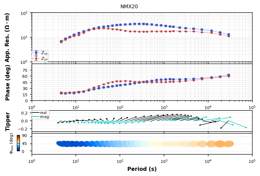
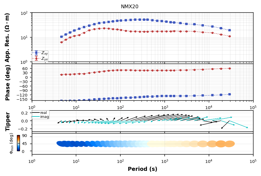
Plot MT Response

The main visualization is plotting the MT response as apparent resistivity and phase, and if there are induction vectors plot them. This also plots the phase tensor ellipses for completeness. You can turn them on and off if you like.

[19]:

plot_response = mt_object.plot_mt_response()

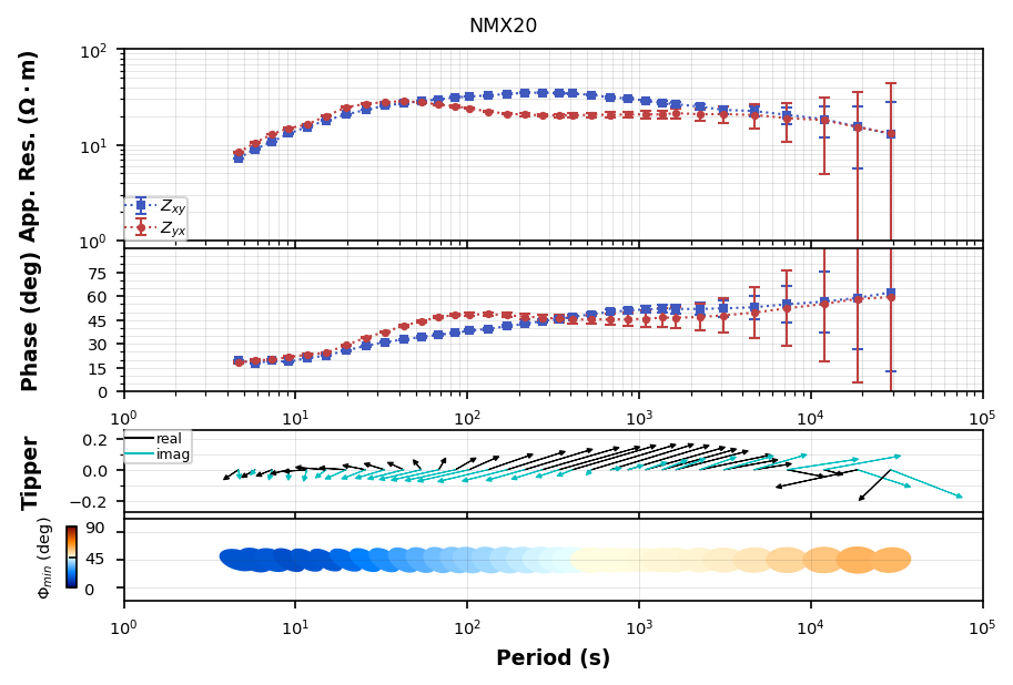
You can plot all 4 components of the impedance tensor

[20]:

plot_response.plot_num = 2
plot_response.fig_num = 2
plot_response.plot()

Plot Phase Tensor component

Sometimes it can be infomrative to plot the phase tensor components and attributes to determine dimensionality.

[21]:

plot_pt = mt_object.plot_phase_tensor()

Plot Penetration Depth

Another diagnostic of your data is to estimate the depth of penetration. This is done through a Niblett-Bostick transformation.

[22]:

plot_nb = mt_object.plot_depth_of_penetration()

Manipulating MT Response

Often you want to manipulate the transfer function by applying a static shift, rotationg, flipping phases, interpolating. There are tools for this.

Rotate

Data rotation helps align the data with geologic structures and optimzing the transfer function to be quasi 2D for modeling.

Geoelectric strike can be estimated from the phase tensor as seen in the plot above. Here this station appears to have a dominant geoelectric strike within the 2D realm is N270E.

Note: All rotations are clockwise assuming that geographic north = 0, and east is 90.

[23]:

rotated = mt_object.rotate(-270, inplace=False)
rotated.plot_phase_tensor()

[23]:

Plotting PlotPhaseTensor

Interpolate

Interpolating data is useful for standardizing a data set for modeling or comparing. Interpolation is done on each component on both real and imaginary parts using a linear interpolation using scipy.signal.interp1d internally within xarray.

Note: Due to some complexities with xarray of removing Nan values a preliminary interpolation is done to interoplate Nan values using using the original period range, then an interpolation is done onto the new period range given. You can change the type of interpolation for the ‘na_interpolate’ and ‘method’.

[24]:

import numpy as np

[25]:

interpolated = mt_object.interpolate(np.logspace(1, 4, 12))

[26]:

interpolated.plot_mt_response()

[26]:

Plotting PlotMTResponse

Static Shift

Static shift is a distortion that affects the apparent resisitivity. We can apply a scalar to shift apparent resistivity up or down.

$\mathbf{Z} = \mathbf{S} * \mathbf{Z}_0$

where:

$\mathbf{S} = \begin{vmatrix} S_{x} \quad S_{x}\\ S_{y} \quad S_{y} \end{vmatrix}$

To remove the static shift multiply by $\mathbf{S}^{-1}$

Note: This assumes that the static shift is given in resistivity coordinates thus the square root of S will be applied.

Note: Numbers great than 1 will move the apparent resisitity down and numbers smaller than 1 will shift apparent resistivity up.

[27]:

static_shifted = mt_object.remove_static_shift(ss_x=1.5)

[28]:

static_shifted.plot_mt_response()

[28]:

Plotting PlotMTResponse

Flip Phase

Occasionally you will compute a transfer function that has phase flipped, usually a coil was hooked ub backwards, or the electric lines were hooked up in reverse. If Hz data were collected an easy way to tell is plotting induction vectors for the survey and seeing if any look flipped. That is a good indication the magnetic channels was flipped. Otherwise check the electric channels. Here we will assume that the Ex was flipped so we flip Zxx and Zxy.

[29]:

flipped = mt_object.flip_phase(zxx=True, zxy=True)
flipped.plot_mt_response()

[29]:

Plotting PlotMTResponse

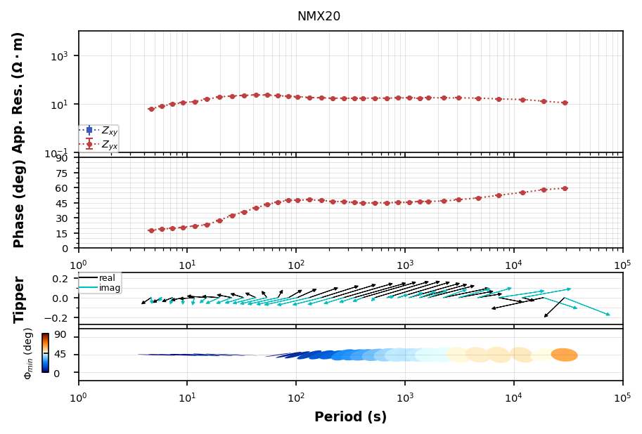
Remove a component

Sometimes data can be terrible for a single component and you may want to remove it before analyzing the data.

[30]:

removed_xy = mt_object.remove_component(zxy=True)
removed_xy.plot_mt_response()

[30]:

Plotting PlotMTResponse

Add White Noise

If you are doing some sensitivity tests or inverting synthetic data adding white noise can be useful. Here we will add 5%

[31]:

adding_white_noise = mt_object.add_white_noise(.05, inplace=False)

[32]:

adding_white_noise.plot_mt_response()

[32]:

Plotting PlotMTResponse

Remove Distortion

Distortion is a pain an usually comes in the form of near surface distortion like a static shift. If you have no other way to estimated distortion, like a TEM measurement or nearby stations a relative estimate can be made using the phase tensor. See Bibby et al., (2005). This basically looks for 1D parts of the transfer function by comparing the TE and TM phases. If the phases match then so should the apparent resistivity. However, knowing the true value of static shift is incomplete and therefore the apparent resistivity curves are pinched together to remove relative static shift.

There might be some issues with uncertainty propagation.

[33]:

distortion_removed = mt_object.remove_distortion(n_frequencies=25)

[34]:

distortion_removed.plot_mt_response()

[34]:

Plotting PlotMTResponse

[ ]: